Discrete Differential Geometry from Scratch

A triangle mesh is a discrete approximation of a smooth surface. Most of the differential geometry of smooth surfaces, such as curvature and the Laplace–Beltrami operator, has a discrete version defined over a vertex and its neighbours. In this project, I implemented these operators and used them for registration, curvature estimation, spectral analysis and smoothing.

I use trimesh to load meshes and answer adjacency queries, and scipy for sparse linear algebra and KD-trees. Everything else is implemented by me, including the Laplacians, curvature, the eigensolve, the ICP variants and the dual construction.

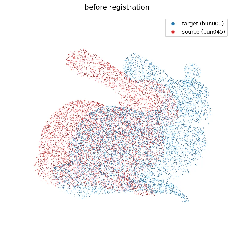
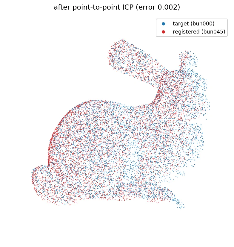
Two scans of the same object taken from different viewpoints need to be aligned before they can be merged. ICP (Iterative Closest Point) does this by alternating between two steps. It pairs each point in one scan with its nearest point in the other, found with a KD-tree, and then solves for the rigid transform that best aligns those pairs. For point-to-point ICP, the best rotation has a closed-form solution from the SVD of the pairs' cross-covariance matrix. Repeating both steps converges to a local optimum.

Point-to-plane ICP measures the distance along the target's surface normal instead of to a single point, which lets points slide along the surface and converges in fewer iterations. With more than two scans, matching each scan against the model built so far works better than matching every scan to the first one, since scans taken far apart share very little surface.

A halfedge structure stores every edge as two directed halfedges, one for each face it borders. Each halfedge knows its opposite halfedge, the next halfedge around its face, and the vertex it starts from, which makes it easy to walk around a face or around the ring of neighbours of a vertex.

I used it to build the dual of a mesh, which places a vertex at the centre of every face and connects the centres of neighbouring faces. For example, the dual of a cube is an octahedron.

Mean curvature can be estimated from the Laplacian of the vertex positions. The uniform Laplacian only uses connectivity, so it reports curvature wherever the triangulation is irregular. The cotangent Laplace–Beltrami operator weights each neighbour by the cotangents of the two angles opposite their shared edge, so it measures the actual surface instead.

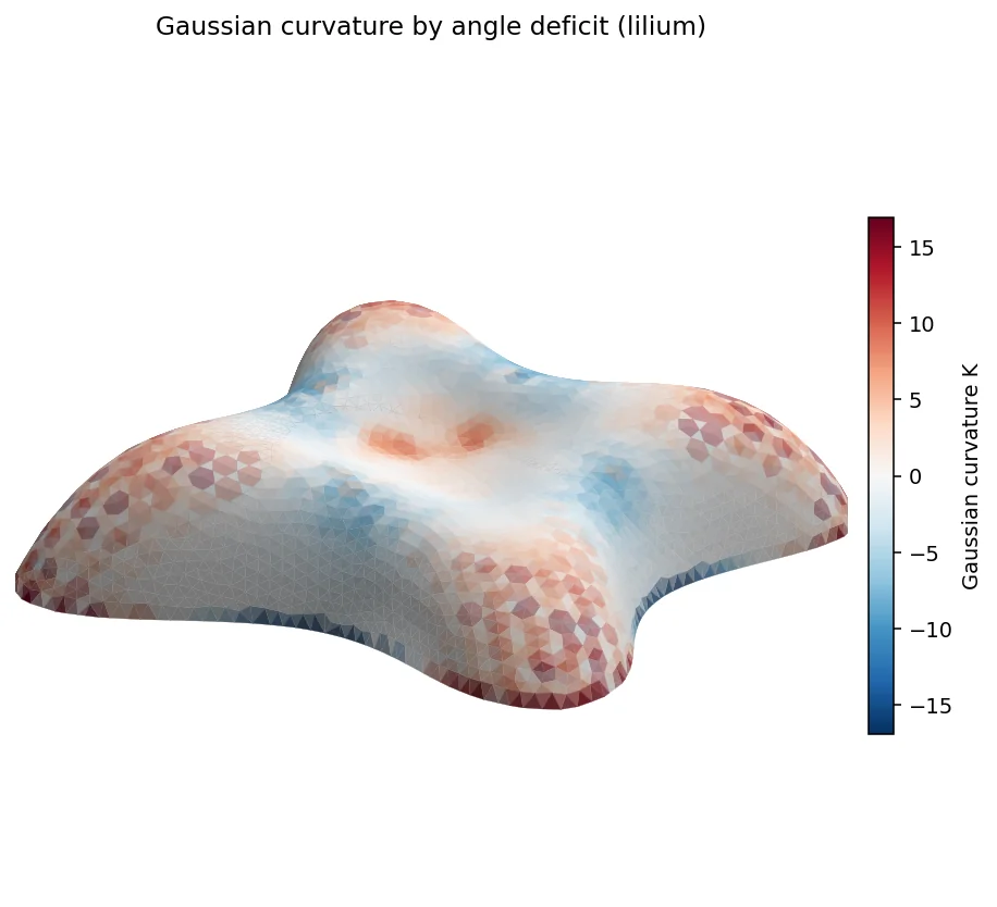
Gaussian curvature is estimated by angle deficit. On a flat surface, the angles around a vertex sum to 2π, so the amount by which they fall short, divided by the area around the vertex, measures how curved the surface is there. It is positive on convex regions and negative at saddles. I validated both against a sphere, where the exact curvature is known.

The eigenvectors of the Laplace–Beltrami operator play the same role on a surface that sines and cosines play for a signal. Eigenvectors with small eigenvalues vary slowly across the surface, and those with large eigenvalues capture fine detail. Projecting the vertex positions onto only the first k eigenvectors is therefore a low-pass filter on the shape. The card image above is the armadillo reconstructed from its first 50 eigenmodes.

The smoothest modes have eigenvalues close to zero, which are slow to find directly. Solving with shift-invert around zero turns them into the largest eigenvalues of the inverted problem, which are much easier to find.

Curvature flow moves every vertex along its mean curvature normal, which smooths the surface by gradually shrinking it. The explicit scheme takes a step of size λ along the Laplacian, which is simple but becomes unstable when λ is too large. The implicit scheme instead solves a sparse linear system for the new positions, which stays stable for any step size.

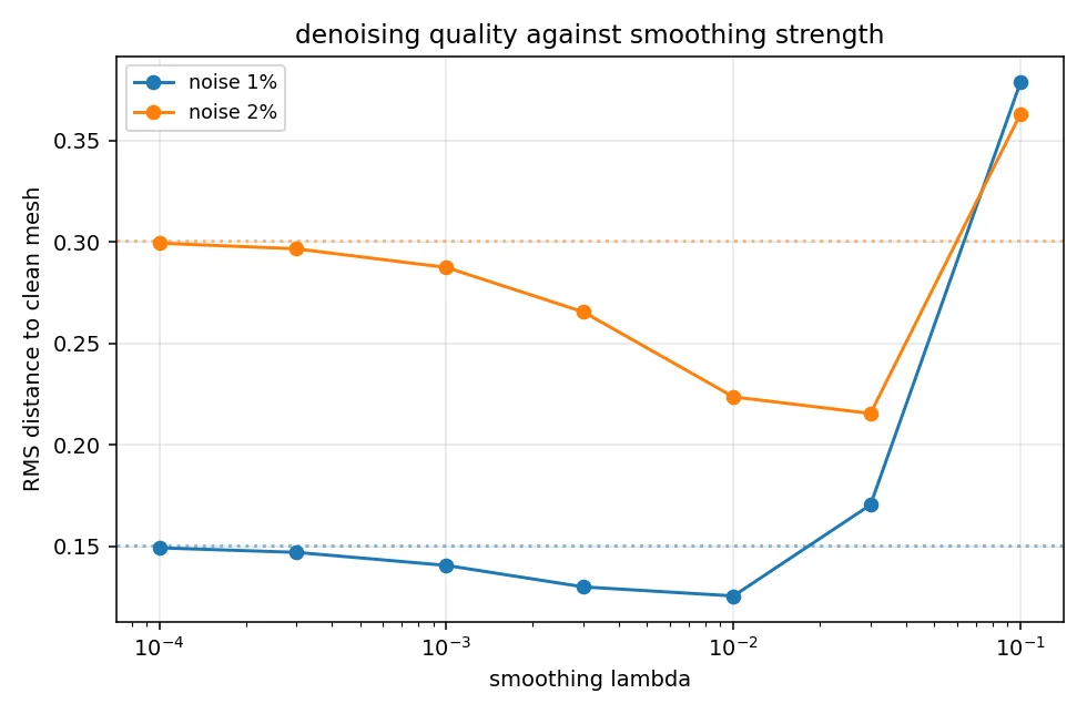
To denoise a mesh, I add noise of a known size and sweep λ. A value that is too small leaves the noise in place, while one that is too large smooths away the shape, and the best value increases with the amount of noise.