Probabilistic Models for Vision

Every method in this repository can be thought of as a likelihood along with a way to search it. In the first half, I build likelihoods and evaluate them against labels. In the second half, I search one over time using a set of particles.

The mixture model fitted in the first part is then used by the tracker in the second part as its appearance model, in place of the template matching used in the original coursework.

I implemented EM, k-means++, log-sum-exp, PCA by SVD, the ROC and AUC, systematic resampling, the condensation loop and every density evaluation myself, without using sklearn.mixture, sklearn.metrics, scipy.stats.multivariate_normal or OpenCV trackers.

The simplest density is a single normal distribution. Maximum likelihood estimation (MLE) picks the parameters that make the data most likely, and MAP adds a prior over those parameters. The Bayesian predictive goes a step further and averages over every possible set of parameters, weighted by how well each one explains the data.

With only a few samples, MLE fits a variance to them and treats it as certain, while the predictive keeps its uncertainty about the parameters, so it generalises much better to new data. As the amount of data grows, the prior matters less and the two converge to the same answer.

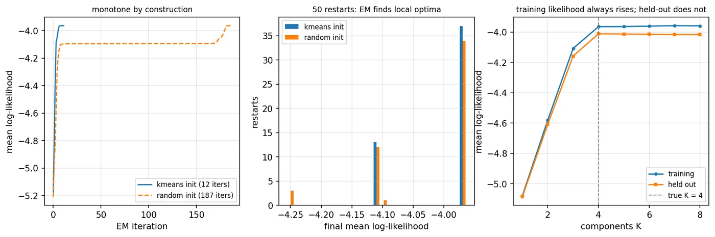
A single normal cannot represent data with several clusters, so I use a mixture of normals. EM fits one by alternating between two steps. The E-step computes how responsible each component is for each point, and the M-step refits each component to the points, weighted by those responsibilities. These probabilities are computed with log-sum-exp to avoid underflow.

The likelihood never decreases between iterations, but EM only finds a local optimum, so I initialise it with k-means++ and run several restarts. To choose the number of components, I compare likelihood on held-out data, since the training likelihood keeps rising with every component added.

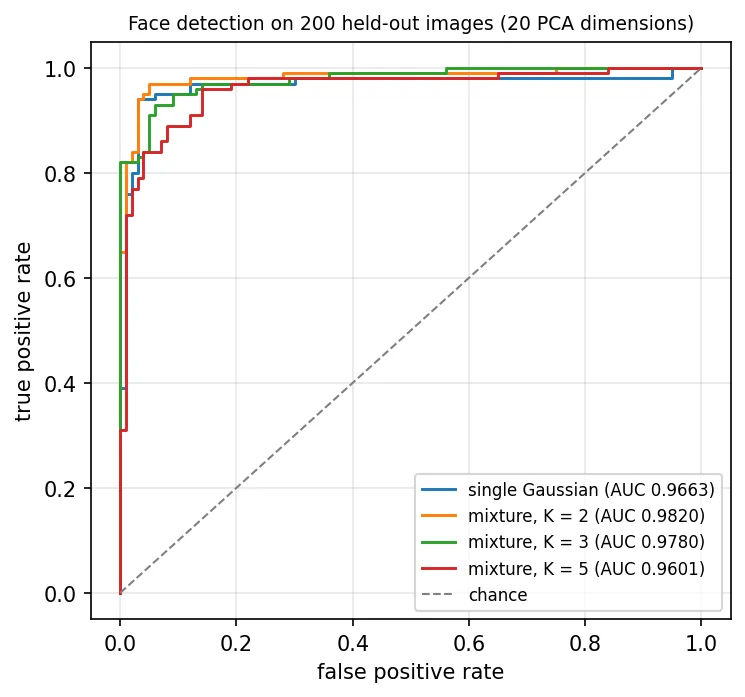
To classify, I fit one density per class and compare their posteriors using Bayes' rule. Sweeping the decision threshold on the ratio of the two posteriors traces out the ROC curve.

For face detection, the images are first projected onto 20 principal components with PCA, since a full covariance over all 10,800 pixel values would need far more parameters than there are training images. The same approach segments skin, by fitting mixtures to the colours of skin and non-skin pixels.

The tracker represents its belief about the object's position as a set of particles. In every frame, each particle is moved by a random walk and weighted by the likelihood of the image at its position, and the set is then resampled in proportion to those weights. This is the condensation algorithm. I use systematic resampling, which has the same expected counts as multinomial resampling but less noise.

For the likelihood, I use the colour mixture fitted with EM, which, unlike a template, does not depend on how the ball is rotated. Neighbouring pixels are not independent evidence, so the summed log likelihood is divided by a temperature to stop a single particle from taking all of the weight.